Chapter 2, Statistical Learning

What is Statistical Learning

Input variables to a statistical model are often called predictors, independent variables, features, or just variables.

Output variable from a statistical model is often called response, or dependent variable.
In essence, statistical learning refers to a set of approaches for estimating f (error term)

Y=f(X)+ε

Why Estimate f

Estimating f is used for prediction and inference.

The prediction accuracy depends on two quantities, reducible error and irreducible error.

The reducible error measure the prediction error as function of X and predicted Y, which by using appropriate statistical learning technique can be reduced.

The irreducible error measure the prediction error as function of ε and the predicted Y. Its irreducible as no matter how well we estimate Y, we cannot reduce the error introduced by ε. The irreducible error may contain unknown variables, variations and variance of the estimated output Y.

The techniques of statistical learning focus on estimating of f with aim of minimizing the reducible error.

The inference task is about understanding the relations between the output and the predictors. Some questions to ask are

• Which predictors have strong influence on Y
• What is the relationship between the response and each predictor
• Is the relation between Y and predictors representable in linear equation or not

Linear models allow for relatively simple and interpretable inference, but may not yield as accurate predictions as some other approaches

Non-Linear models provide quite accurate predictions for Y , but this comes at the expense of a less interpretable model for which inference is more challenging

How F is estimated

The process here is to observe training data and train a statistical model to find Y ≈ f(X). There are two methods to do so parametric and nonparametric.

Parametric methods involve two step model based approach

• Define and select a linear model f(X)=WX+b
• Select a procedure for fitting the train data to the selected model. Example of such procedure is least squares method.

Choosing close model to the true function of f is challenging. Choosing a too far model would result in poor estimation.

Overfitting is a phenomena when the model fits much to the noise in the training data instead of generalizing to capture the underlying f.

Nonparametric methods do not make explicit assumptions about the functional form of f. Instead they seek an estimate close to the training data without being too rough or too wiggly. Advantage of such methods is ability to cover wide range of shapes of f, though this requires training data way more than parametric methods to generalize.

Usually restrictive, simple and linear models are more suitable than flexible models for inference tasks.

Regression problems are about predicting an quantitative response while the classification problems are about predicting a qualitative response.

Model Accuracy Assessment

In regression problems mean square error is commonly used.

Mean Square Error

 

Chapter 1, Introduction

Statistical learning refers to a vast set of tools for understanding data. Types of statistical learning:

• Supervised statistical learning involves building a statistical model for predicting, or estimating, an output based on one or more inputs
• Unsupervised statistical learning, there are inputs but no supervising output; nevertheless we can learn relationships and structure from such data

Linear regression is used for predicting quantitative values, such as an individual’s salary

Statistical Learning History:

• Around 1900, Legendre and Gauss published method of least squares papers (a form of linear regression)
• In 1936, Fisher proposed linear discriminant analysis for predicting qualitative regression problems.
• In 1940, various authors proposed logistic regression for solving the regression problem
• In the early 1970s, Nelder and Wedderburn coined the term generalized linear models for an entire class of statistical learning methods that include both linear and logistic regression as special cases.
• In 1970, many linear models were available however, fitting a nonlinear relationship was computationally infeasible at that time.
• In 1980, the computing technology had improved so it can solve nonlinear problems.
• In mid 1980, Breiman, Friedman, Olshen and Stone introduced classification and regression trees, and were among the first to demonstrate the power of a detailed practical implementation of a method, including cross-validation for model selection
• In 1986, Hastie and Tibshirani coined the term generalized additive models for a class of nonlinear extensions to generalized linear models
• In the past years, progress on statistical learning techniques and tools has been marked by the increasing availability of powerful and relatively user-friendly software

Udacity Deep Learning Course Summary

Introduction

Logistic Classifier (Linear Classifier): Takes an input (image pixels) and applies a linear function to them to make predictions.

Linear Function: WX + b = Y, where W is weight matrix, X is input matrix, b is bias and Y is output matrix. The W and b terms are the trained values.

Softmax: is a way to transform scores into probabilities. Increasing the number of training data set would make the classifier more confident and discriminate individual classes clearly.

One-Hot Encoding is when the correct class has probability of 1.0 and other classes 0 probability. This technique is not efficient on large number of classes. The benefit is measuring cross-entropy is easy.

Multinomial Logistic Classification is setting where input is feeded to linear model to logistic to softmax to one-hot encoding.

Gradient Descent is the technique used for finding the value to minimize the loss function. A correct simulation should update Theta0 and Theta1 at same time not after each other.

Learning Rate is variable that controls how big a step the gradient descent takes downhill.

For a Local Minimum the slope is going to be zero and this will result in 0 for derivative term which would result in same value of theta.

Training Dataset is the data set that the classifier uses to train on.

Validation Dataset is the data set used for validation and also it’s possible to reconstruct this dataset until the classifier looks like generalized.

Test Dataset is the data set used for real testing. Data samples that the classifier never saw before.

Rule of 30 is an idea to measure if improvements in the classification model is significant or not.

Usually models use more 30K examples for validation to assure significance. Whenever there’s an improvements more than 0.1% this will be significant, which makes measuring the improvements easy.

The main problem with Gradient Descent is that it’s gets calculated for each example in the training data set, and the derivative term takes long time from processing standpoint. This problem will arise in scalability scenarios where the training data set is huge.

To overcome the scalability and performance issues of gradient descent, using a small random data (to calculate its average loss) set out of the training data set with small learning rate overcomes this problem. That technique is called Stochastic Gradient Descent (SAG).

Use running average of the loss instead of relying solely on the current instance helps reducing the number of steps to converge. This is called momentum technique

Using lower learning rate usually tends to get a more accurate classifier.

Stochastic Gradient Descent Parameters:

• Initial Learning Rate: the initial value for learning rate
• Learning Rate Decay: how much learning rate should increase
• Momentum: the running average of the loss
• Batch Size: the random sample used by SGD
• Weight Initialization

ADAGRAD is a technique that eliminates couple of SGD parameters and require batch size and weights only.

Deep Neural Networks

Rectified Linear Units (RELU): non-linear function that’s y=x for y > 0 and 0 otherwise.

Backpropagation is used to calculate the gradient of the cost function to update the weights.

Deep Learning is about adding more hidden layers to the model. This helps because of:

• Parameter efficiency: uses few parameters but goes deeper.
• Model Abstraction: going deeper results into layers that learn more generalized and useful shapes, like geometric shape instead of line

Why deep learning has not been used before?

• Deep learning, requires large dataset which has been available recently
• Better regularization techniques

Regularization is a technique used to prevent from overfitting

Avoid overfitting:

• Early termination for the training using validation set as soon as the performance stops improving
• Using regularization techniques
  • Adding L2 for the weights vector
  • Using Dropout

Dropout (by Geoffrey Hinton) is a regularization technique used to prevent overfitting by stochastically turning off activations for hidden layers. This forces the network not to rely on a specific activation in its training and it learns redundant representation for everything across the input data.

Redundant representations results in a network that need some consensus technique to decide the result.

Convolutional Neural Network

If the structure of the input is known, then there’s a chance to reduce the NN complexity by relying on such fact. For example, if the input is a colored letter then the NN can be simplified by using grayscale instead of adding the colors complexity to the NN.

Features that do not change across time, space or everywhere are called statistical invariant. For example, translation invariance is used to simplify the NN by disregard learning the location of the object in an image.

Weight sharing is used to simplifying learning in a NN by utilizing statistical invariance.

CNN (by Yann LeCun) are NN that share their parameters across the space.

Convolution is the process of applying a mask to a NN in convolution pattern (like image filters) to a given image. This would result into a matrix that has different width, height and depth from the original image.

The layer’s parameters consist of a set of learnable filters (or kernels/patches), which have a small receptive field, but extend through the full depth of the input volume.

An RGB image has three feature maps each corresponds to one color intensity.

Stride is the number of pixels shifted each time the filter is moved

Valid padding is way to cut the image as the size of the filter

Same padding is way to pad zeros at the edge of the image to keep sizes same.

Striding reduces the feature map size but it’s very aggressive and sometimes result in loss of data.  Pooling is a technique used for combining information for an image sample. Two common pooling techniques are max pooling and average pooling.

1×1 convolution is a way to reduce the dimensionality of the NN in a simple way.

Recurrent Neural Network is a NN that’s used with temporal classification/prediction problems.

Long Short Term Memory (LSTM) is a version from RNN that’s being used widely.

Introduction to the Introduction

Download this Article

What Is Machine Learning?

We do not know exactly which people are likely to buy a particular product, or which author to suggest to people who enjoy reading Hemingway. If we knew, we would not need any analysis of the data; we would just go ahead and write down the code. But because we do not, we can only collect data and hope to extract the answers to these and similar questions from data.

We do believe that there is a process that explains the data we observe. Though we do not know the details of the process underlying the generation of data-for example, consumer behavior-we know that it is not completely random. People do not go to supermarkets and buy things at random. When they buy beer, they buy chips; they buy ice cream in summer and spices for Ghihwein in winter. There are certain patterns in the data.

We may not be able to identify the process completely, but we believe we can construct a good and useful approximation. That approximation may not explain everything, but may still be able to account for some part of the data. We believe that though identifying the complete process may not be possible, we can still detect certain patterns or regularities. This is the niche of machine learning.

Application of machine learning methods to large databases is called data mining.

But machine learning is not just a database problem; it is also a part of artificial intelligence. To be intelligent, a system that is in a changing environment should have the ability to learn. If the system can learn and adapt to such changes, the system designer need not foresee and provide solutions for all possible situations.

The model may be predictive to make predictions in the future, or descriptive to gain knowledge from data, or both.

Examples of Machine Learning Applications

Learning Associations:

In the case of retail-for example, a supermarket chain-one application of machine learning is basket analysis, which is finding associations between products bought by customers: If people who buy X typically also buy Y, and if there is a customer who buys X and does not buy Y, he or she is a potential Y customer. Once we find such customers, we can target them for cross-selling.

In finding an association rule, we are interested in learning a conditional probability of the form where is the product we would like to condition on , which is the product or the set of products which we know that the customer has already purchased.

Let us say, going over our data, we calculate that = 0.7. Then, we can define the rule:

70 percent of customers who buy beer also buy chips

We may want to make a distinction among customers and toward this, estimate where is the set of customer attributes, for example, gender, age, marital status, and so on, assuming that we have access to this information.

Classification:

In credit scoring (Hand 1998), the bank calculates the risk given the amount of credit and the information about the customer. The information about the customer includes data we have access to and is relevant in calculating his or her financial capacity-namely, income, savings, collaterals, profeSSion, age, past financial history, and so forth. The bank has a record of past loans containing such customer data and whether the loan was paid back or not. From this data of particular applications, the aim is to infer a general rule coding the association between a customer’s attributes and his risk. That is, the machine learning system fits a model to the past data to be able to calculate the risk for a new application and then decides to accept or refuse it accordingly.

This is an example of a classification problem where there are two classes: low-risk and high-risk customers. The information about a customer makes up the input to the classifier whose task is to assign the input to one of the two classes.

A discriminant function, is a function that separates the examples of different classes. This type of applications is used for prediction.

There are many applications of machine learning in pattern recognition. One is optical character recognition, which is recognizing character codes from their images.

In medical diagnosis, the inputs are the relevant information we have about the patient and the classes are the illnesses. The inputs contain the patient’s age, gender, past medical history, and current symptoms. Some tests may not have been applied to the patient, and thus these inputs would be missing. Tests take time, may be costly, and may inconvience the patient so we do not want to apply them unless we believe that they will give us valuable information. In the case of a medical diagnosis, a wrong decision may lead to a wrong or no treatment, and in cases of doubt it is preferable that the classifier reject and defer decision to a human expert.

Learning also performs compression in that by fitting a rule to the data, we get an explanation that is simpler than the data, requiring less memory to store and less computation to process. Once you have the rules of addition, you do not need to remember the sum of every possible pair of numbers.

Another use of machine learning is outlier detection, which is finding the instances that do not obey the rule and are exceptions. In this case, after learning the rule, we are not interested in the rule but the exceptions not covered by the rule, which may imply anomalies requiring attention for example, fraud.

Regression:

Let us say we want to have a system that can predict the price of a used car. Inputs are the car attributes-brand, year, engine capacity, milage, and other information-that we believe affect a car’s worth. The output is the price of the car. Such problems where the output is a number are regression problems.

Both regression and classification are supervised learning problems where there is an input, X, an output, Y, and the task is to learn the mapping from the input to the output. The approach in machine learning is that we assume a model defined up to a set of parameters: .

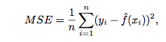
where is the model and are its parameters. is a number in regression and is a class code (e.g., 0/1) in the case of classification. is the regression function or in classification, it is the discriminant function separating the instances of different classes. The machine learning program optimizes the parameters, , such that the approximation error is minimized, that is, our estimates are as close as possible to the correct values given in the training set.

One can envisage other applications of regression where one is trying to optimize a function. Let us say we want to build a machine that roasts coffee. The machine has many inputs that affect the quality: various settings of temperatures, times, coffee bean type, and so forth. We make a number of experiments and for different settings of these inputs, we measure the quality of the coffee, for example, as consumer satisfaction. To find the optimal setting, we fit a regression model linking these inputs to coffee quality and choose new points to sample near the optimum of the current model to look for a better configuration. We sample these points, check quality, and add these to the data and fit a new model. This is generally called response surface design.

Unsupervised Learning:

In supervised learning, the aim is to learn a mapping from the input to an output whose correct values are provided by a supervisor. In unsupervised learning, there is no such supervisor and we only have input data. The aim is to find the regularities in the input. There is a structure to the input space such that certain patterns occur more often than others, and we want to see what generally happens and what does not. In statistics, DENSITY ESTIMATION this is called density estimation.

One method for density estimation is clustering where the aim is to find clusters or groupings of input. In the case of a company with a data of past customers, the customer data contains the demographic information as well as the past transactions with the company, and the company may want to see the distribution of the profile of its customers, to see what type of customers frequently occur. In such a case, a clustering model allocates customers similar in their attributes to the same group, providing the company with natural groupings of its customers. Once such groups are found, the company may decide strategies, for example, services and products, specific to different groups. Such a grouping also allows identifying those who are outliers, namely, those who are different from other customers, which may imply a niche in the market that can be further exploited by the company.

An interesting application of clustering is in image compression. In this case, the input instances are image pixels represented as RGB values. A clustering program groups pixels with similar colors in the same group, and such groups correspond to the colors occurring frequently in the image. If in an image, there are only shades of a small number of colors and if we code those belonging to the same group with one color, for example, their average, then the image is quantized. Let us say the pixels are 24 bits to represent 16 million colors, but if there are shades of only 64 main colors, for each pixel, we need 6 bits instead of 24. For example, if the scene has various shades of blue in different parts of the image, and if we use the same average blue for all of them, we lose the details in the image but gain space in storage and transmission. Ideally, one would like to identify higher-level regularities by analyzing repeated image patterns, for example, texture, objects, and so forth. This allows a higher-level, simpler, and more useful description of the scene, and for example, achieves better compression than compressing at the pixel level.

One application area of computer science in molecular biology is alignment, which is matching one sequence to another. This is a difficult string matching problem because strings may be quite long, there are many template strings to match against, and there may be deletions, insertions, and substitutions. Clustering is used in learning motifs, which are sequences of amino acids that occur repeatedly in proteins. Motifs are of interest because they may correspond to structural or functional elements within the sequences they characterize. The analogy is that if the amino acids are letters and proteins are sentences, motifs are like words, namely, a string of letters with a particular meaning occurring frequently in different sentences.

Reinforcement Learning:

In some applications, the output of the system is a sequence of actions. In such a case, a single action is not important; what is important is the policy that is the sequence of correct actions to reach the goal. an action is good if it is part of a good policy. In such a case, the machine learning program should be able to assess the goodness of policies and learn from past good action sequences to be able to generate a policy. Such learning methods are called reinforcement learning algorithms.

A good example is game playing where a single move by itself is not that important; it is the sequence of right moves that is good. A move is good if it is part of a good game playing policy.

A robot navigating in an environment in search of a goal location is another application area of reinforcement learning. At any time, the robot can move in one of a number of directions. After a number of trial runs, it should learn the correct sequence of actions to reach to the goal state from an initial state, doing this as quickly as possible and without hitting any of the obstacles.

One factor that makes reinforcement learning harder is when the system has unreliable and partial sensory information. For example, a robot equipped with a video camera has incomplete information and thus at any time is in a partially observable state and should decide taking into account this uncertainty. A task may also require a concurrent operation of multiple agents that should interact and cooperate to accomplish a common goal. An example is a team of robots playing soccer.

Notes

Induction is the process of extracting general rules from a set of particular cases.

In statistics, going from particular observations to general descriptions is called inference and learning is called estimation. Classification is called discriminant analysis in statistics.

In engineering, classification is called pattern recognition and the approach is nonparametric and much more empirical.

Machine learning is related to artificial intelligence (Russell and Norvig 1995) because an intelligent system should be able to adapt to changes in its environment.

Data mining is the name coined in the business world for the application of machine learning algorithms to large amounts of data (Weiss and Indurkhya 1998). In computer science, it is also called knowledge discovery in databases (KDD).

Chapter’s Important Keywords:

1. Machine Learning.
2. Data Mining.
3. Descriptive Model.
4. Predictive Model.
5. Association Rule.
6. Classification.
7. Discriminant Function.
8. Knowledge Extraction.
9. Compression.
10. Outlier Detection.
11. Supervised Learning.
12. Response Surface Design.
13. Density Estimation.
14. Clustering.
15. Reinforcement Learning.
16. Partially Observable State.
17. Induction.
18. Inference.
19. Estimation.
20. Discriminant Analysis.
21. Knowledge Discovery in Databases.

Preface

Machine learning is about programming computers to optimize a performance
criterion using example data or past experience.

Examples of Machine Learning

1. Recognition of spoken speech. That is, converting the acoustic speech signal to an ASCrr text.
   
2. Consider routing packets over a computer network. The path maximizing the quality of service from a source to destination changes continuously as the network traffic changes. A learning routing program is able to adapt to the best path by monitoring the network traffic.
   
3. Intelligent user interface that can adapt to the biometrics of its user, namely, his or her accent, handwriting, working habits, and so forth.
   
4. Retail companies analyze their past sales data to learn their customers’ behavior to improve customer relationship management.
   
5. Financial institutions analyze past transactions to predict customers’ credit risks.
   
6. Robots learn to optimize their behavior to complete a task using minimum resources.
   
7. In bioinformatics, the huge amount of data can only be analyzed and knowledge be extracted using computers.
   
8. Cars that can drive themselves under different road and weather conditions.
   
9. Phones that can translate in real time to and from a foreign language.
   
10. Autonomous robots that can navigate in a new environment, for example, on the surface of another planet.
    

 

The book I’m reading, discusses many methods that have their bases in different fields; statistics, pattern recognition, neural networks, artificial intelligence, signal processing, control, and data mining.

 

Multilayer Perceptron

• Multilayer perception stands for a neural network with one or more hidden layer.
• Properties of multilayer neural networks:
  • The model of each neuron in the network includes a nonlinear activation function that’s differentiable.
  • Network contains one or more hidden layer.
  • Network exhibits a high degree of connectivity through its synaptic weights.
• Common deficiencies in multilayer neural networks:
  • Theoretical analysis of MLNN is difficult to undertake.
    • This comes from the nonlinearity and high connectivity of the network.
  • Harder efforts are required for visualizing the learning process.
    • This comes from the existence of several layers in the network.
• Back propagation algorithm is used to train MLNN. The training proceeds in two phases:
  • In the forward phase, the synaptic weights of the network are fixed and the input signal is propagated through the network layer by layer until it reaches the output.
  • In the backward phase, an error signal is produced by comparing the output of the network with a desired response. The resulting error signal is propagated through the network, layer by layer but the propagation is performed in the
    backward direction. In this phase successive adjustments are applied to the synaptic weights of the network.
• The term “back propagation” appeared after 1985 when the term was popularized through the publication of the book “Parallel Distribution Processing” by Rumelhard and McClelland.

• Two kinds of signals exist in MLP (Multilayer Perceptron):
  • Function Signals (Input Signal):
    • It’s an input signal that comes in at the input end of the network, propagates forward (neuron by neuron) through the network and emerges at the output end of the network as output signal.
    • We called it Function Signals because:
      • It’s presumed to perform a useful function at the output of the network.
      • The neuron’s signal is calculated as a function of the input signal(s) and associated weights.
  • Error Signals:
    • It originates at an output neuron of the network and propagates backward (layer by layer) through the network.
    • We called it Error Signal because:
      • It’s computation by every neuron of the network involves an error-dependent function.
• Each hidden or output neuron of a multilayer perceptron is designed to perform two computations:
  • Computation of function signal, which is expressed as a continuous nonlinear function of the input signal and synaptic weights associated with that neuron.
  • Computation of an estimate of the gradient vector which is needed for the backward pass through the network.
    • Gradient vector: the gradients of the error surface with respect to the connected weights of the inputs of a neuron.
• Function of Hidden Neurons:
  • Hidden neurons act as feature detector.
  • The hidden neurons are able to discover the salient features that characterize training data.
  • They do so by performing a nonlinear transformation on the input data into a new space called feature space
  • In feature space pattern classification task is more simplified and the classes are more separated.
  • This function is the main difference between Rosenblatt’s perceptron and Multilayer Neural Networks.
• Credit Assignment Problem:
  • Credit-Assignment problem is the problem of assigning credit or blame for overall outcomes to each of the internal decisions made by the hidden computational units of the learning system. Because as we know those decisions are responsible for the overall outcomes in the first place.
  • Error-correction learning algorithm is not suitable for resolving the credit-assignment problem for MLNN because we can’t just judge on the output neurons where hidden layers play a big role in its decision.
  • Back propagation algorithm is able to solve the credit-assignment problem in an elegant manner.

  Batch Learning
  

• Before we start in describing the algorithm you want to introduce some equations that are found in page 157.
• Batch Learning is a supervised learning algorithm. The learning algorithm is performed after the presentation of all the N examples in the training samples that constitutes one epoch of training.
• Adjustments to the synaptic weights are made on an epoch-by-epoch basis.
• With method of gradient descent used to perform training we’ve these 2 advantages:
  • Accurate estimation.
  • Parallelization of learning process.
• From practical perspective, batch learning suffers from the storage requirements.
• In statistical context, batch learning can be viewed as a form of statistical inference. It’s therefore well studied for solving nonlinear regression problems.

Online Learning

• Online method of supervised learning, adjustments to the synaptic weights of the multilayer perceptron is performed example-by-example basis. The cost function to be minimized is therefore the total instantaneous error energy.
• Such algorithm is not suitable for parallelization of the learning process.
• Sometimes online learning is called stochastic method.
• Advantages of online learning:
  • This stochasticity has the desirable effect of making it less likely for the learning process to be trapped in a local minimum.
  • Moreover, online learning requires less storage than batch learning.
  • Also, if the training data is redundant, the online learning benefits from this redundancy to improve its learning.
  • Finally, in online learning you are able to track small changes in training data especially if the data environment is non-stationary.
  • It’s simple to implement.
  • Provides effective solutions to large –scale and difficult classification problems.

The Back Propagation Algorithm

• First you should read the mathematical derivation of the algorithm in pages 195-161.
• The key factor involved in the calculation of the weight adjustment is the error signal at the output neuron j. As we see the credit-assignment problem arises here. In this context we may identify two distinct cases:
  • Case #1: Neuron j is an output node:
    • The error signal is supplied to the neuron by its own from equation:
    • • Where .
  • Case #2: Neuron j is a hidden node:
    • When a neuron j is located in a hidden layer of the network, there’s no specified desired response for that neuron.
    • Accordingly, the error signal for a hidden neuron would have to be determined recursively and working backwards in terms of the error signals of all the neurons to which that hidden neuron connected.
    • The final back-propagation formula for the local gradient
      • Where k represents the number of neurons that are connected to hidden neuron j.
    • To know the derivation kindly refer to page 162-163.
• As a summary the correction is applied to the synaptic weight connecting neuron I to j is defined by:
• Any activation function that is used in multilayer neural networks should be continuous.
• The most commonly used activation function is sigmoidal nonlinearity. Two forms of which are described here:
  • Logistic Function: .
  • Hyperbolic Tangent Function: .
• Learning Parameter:
  • The smaller we make, the smaller changes to synaptic weights in the network will be from one iteration to the next and the smoother will be the trajectory in the network weight space.
  • On the other hand if we make to large in order to speed up the rate of learning, the resulting larges changed in synaptic weights assume such for that the network may become unstable (i.e. oscillatory).
  • A simple method of solving this problem is by including a momentum term, as shown by:
    • ,
    • Where usually positive number is called momentum constant.
    • Also, is the unit-time delay operator,
    • The above equation is called generalized delta rule. Special case here is applied when .
  • The inclusion of momentum in back-propagation algorithm has stability effect in directions that oscillate in sign.
  • The momentum term may also have the benefit of preventing the learning process from terminating in a shallow local minimum on the error surface.
  • In reality the learning rate parameter in connection dependent such that each connection has .
• Stopping Criteria:
  • In general back-propagation algorithm can’t be shown to converge and there are no well defined criteria for stopping it operation.
  • We may formulate a sensible convergence criterion for back-propagation learning as follows (Kramer and Sangiovanni-Vincentelli 1989):
    • The back-propagation algorithm is considered to have converged when the Euclidean norm of the gradient vector reaches a sufficiently small gradient threshold.
  • The drawback of this criterion is that, for successful trails, learning times may be long. Also, it requires the computation of the gradient vector g(w).
  • Another criterion:
    • The back-propagation algorithm is considered to have converged when the absolute rate of change in the average squared error per epoch is sufficiently small
      (ranges from 0.1 to 1 percent/epoch).
  • Another theoretical criterion:
    • After each learning iteration, the network is tested for it generalization performance. The learning process stops when the generalization performance is adequate or peaked.
• Note that in each training epoch the samples should be picked randomly.

Designing a neural network with back-propagation algorithm is more of an art than a science

• Heuristics for making back-propagation algorithm perform better:
  • Stochastic update is recommended over batch update.
  • Maximizing the information context.
    • This is done by:
      • Use an example that results in the largest training error.
      • Use an example that is radically different from all those previously worked.
  • Activation Function.
    • It’s preferred to use a sigmoid activation function that’s an odd function in its arguments.
    • The hyperbolic sigmoid function is the recommended one.
    • 175-See the useful properties of hyperbolic sigmoid function.
  • Target values:
    • It’s recommended that target values (desired) be chosen within the range of the sigmoid activation function.
  • Normalizing the inputs.
    • Each input variable should be preprocessed so that its mean value, averaged over the entire training samples, is close or equal to zero.
    • In order to accelerate the back-propagation learning process, the normalization of the inputs should also include two other measures:
      • The input variables contained in the training set should be uncorrelated; this can be done by using principal-component analysis.
      • The decorrelated input variables should be scaled so that their covariances are approximately equal
    • Here we’ve 3 normalization steps:
      • Mean removal.
      • Decorrelation.
      • Covariance equalization.

• Weights initialization.
• Learning from hints.
  • This is achieved by including prior knowledge to the system.
• Learning Rates.
  • All neurons in the multilayer should learn at the same rate, except for that at the last layer, the learning rate should be assigned smaller value than that of the front layers.

Generalization

• A network is said to generalize well when the network input-output mapping is correct (or nearly so) for the test data.
• The learning process may be viewed as “curve fitting” problem. Thus, generalization is performed by the interpolation made by the network.
• Memorization in a neural network usually leads to bad generalization. “Memorization” is essentially a “look-up table”, which implies that the input-output mapping computed by the neural network is not smooth.
• Generalization is influenced by three factors:
  • Size of training sample and how they represent the environment of interest.
  • Architecture of the neural network.
  • Physical complexity of the problem at hand.
• In practice, good generalization is achieved if we the training sample size, N, satisfies:

 

• Where:
  • W is the total number of free parameters (i.e. synaptic weights and basis) in the network.
  • denotes the fraction of classification errors permitted on test data.

Cross Validation

• In statistics, cross-validation randomly divides the available data set into:
  • Training Data:
    • Estimate Subset: used to select the model.
    • Validation Subset: used to test or validate the model.
  • Testing Data.
• However, this best model may be overfitting the validation data.
• Then, to guard against this possibility, the generalization performance is measured on the test set, which is different from the validation subset.
• Early-Stopping Method (Holdout Method):
  • Validation Steps:
    • The training is stopped periodically, i.e., after so many epochs, and the network is assessed using the validation subset where the backward mode is disabled.
    • When the validation phase is complete, the estimation (training) is resumed for another period, and the process is repeated.
    • The best model (free parameters) is that at the minimum validation error.
  • Here we should take care of not going into local minima because of the validation-set.
• Variant of Cross-Validation (Multifold Method):
  • Validation Steps:
    • Divide the data set of N samples into K subsets, where K > 1.
    • The network is validated in each trial using a different subset. After training the network using the other subsets.
    • The performance of the model is assessed by averaging the squared error under validation over all trials.
  • A special case of this method is called “leave-one out method“, where examples are used to train the model, and the model is validated by testing it on the example that left out.
  • Disadvantage of this method is that it requires an excessive amount of computation.
  • Figure below demonstrates the division of the samples. Where the shaded square denotes the validation set.

• Questions:
  • What we mean by differentiable function?
    • It’s a continuous function (i.e. not discrete function).
  • What are benefits of differentiable functions?
    • We are able to use it to find the gradient of the activation function in terms on local induced field.
  • 155- “It’s presumed to perform a useful function at the output of the network”. Here author mean performing an activation function at output layer? Or he means that the output signal will lead us to do some function?
    • Because it gives us the network response (this is the function).
  • 155-I need graphical and mental explanation about “the gradients of the error surface with respect to the weights connected”
  • 158-description realization of the learning curve process.
    • He means the difference between Online and Batch.
  • 158-How “parallelization of learning process” exists in the batch learning process?
    • Distribute the computation of error for each sample and then combine them.
  • 158- “In statistical context, batch learning can be viewed as a form of statistical inference. It’s therefore well studied for solving nonlinear regression problems“. Discussion is required here.
  • 159-Why batch learning doesn’t benefit from redundancy?
  • 159-How we can track small changes in “training data”? Should it be in “synaptic weights”
    • Because it’s sensitive whereas the batch looks for the global changes.
  • 161-What’s local gradient?
    • It’s the synaptic weight that presents the local minimum for the current neuron.
  • 163- I need to know the mathematical differentiation steps of equation 4.23.
  • 169- “The drawback of this criterion is that, for successful trails, learning times may be long. Also, it requires the computation of the gradient vector g(w). What’s the drawback here in calculating g(w)?!
    • Well, I think that it’s computationally expensive to compute it each epoch.
  • 178-What’s meant by saturation?
  • 177-What’s meant by uncorrelated data?

Multilayer Perceptron

• Multilayer perception stands for a neural network with one or more hidden layer.
• Properties of multilayer neural networks:
  • The model of each neuron in the network includes a nonlinear activation function that’s differentiable.
  • Network contains one or more hidden layer.
  • Network exhibits a high degree of connectivity through its synaptic weights.
• Common deficiencies in multilayer neural networks:
  • Theoretical analysis of MLNN is difficult to undertake.
    • This comes from the nonlinearity and high connectivity of the network.
  • Harder efforts are required for visualizing the learning process.
    • This comes from the existence of several layers in the network.
• Back propagation algorithm is used to train MLNN. The training proceeds in two phases:
  • In the forward phase, the synaptic weights of the network are fixed and the input signal is propagated through the network layer by layer until it reaches the output.
  • In the backward phase, an error signal is produced by comparing the output of the network with a desired response. The resulting error signal is propagated through the network, layer by layer but the propagation is performed in the
    backward direction. In this phase successive adjustments are applied to the synaptic weights of the network.
• The term “back propagation” appeared after 1985 when the term was popularized through the publication of the book “Parallel Distribution Processing” by Rumelhard and McClelland.

• Two kinds of signals exist in MLP (Multilayer Perceptron):
  • Function Signals (Input Signal):
    • It’s an input signal that comes in at the input end of the network, propagates forward (neuron by neuron) through the network and emerges at the output end of the network as output signal.
    • We called it Function Signals because:
      • It’s presumed to perform a useful function at the output of the network.
      • The neuron’s signal is calculated as a function of the input signal(s) and associated weights.
  • Error Signals:
    • It originates at an output neuron of the network and propagates backward (layer by layer) through the network.
    • We called it Error Signal because:
      • It’s computation by every neuron of the network involves an error-dependent function.
• Each hidden or output neuron of a multilayer perceptron is designed to perform two computations:
  • Computation of function signal, which is expressed as a continuous nonlinear function of the input signal and synaptic weights associated with that neuron.
  • Computation of an estimate of the gradient vector which is needed for the backward pass through the network.
    • Gradient vector: the gradients of the error surface with respect to the connected weights of the inputs of a neuron.
• Function of Hidden Neurons:
  • Hidden neurons act as feature detector.
  • The hidden neurons are able to discover the salient features that characterize training data.
  • They do so by performing a nonlinear transformation on the input data into a new space called feature space
  • In feature space pattern classification task is more simplified and the classes are more separated.
  • This function is the main difference between Rosenblatt’s perceptron and Multilayer Neural Networks.
• Credit Assignment Problem:
  • Credit-Assignment problem is the problem of assigning credit or blame for overall outcomes to each of the internal decisions made by the hidden computational units of the learning system. Because as we know those decisions are responsible for the overall outcomes in the first place.
  • Error-correction learning algorithm is not suitable for resolving the credit-assignment problem for MLNN because we can’t just judge on the output neurons where hidden layers play a big role in its decision.
  • Back propagation algorithm is able to solve the credit-assignment problem in an elegant manner.

   

  Batch Learning
  

• Before we start in describing the algorithm you want to introduce some equations that are found in page 157.
• Batch Learning is a supervised learning algorithm. The learning algorithm is performed after the presentation of all the N examples in the training samples that constitutes one epoch of training.
• Adjustments to the synaptic weights are made on an epoch-by-epoch basis.
• With method of gradient descent used to perform training we’ve these 2 advantages:
  • Accurate estimation.
  • Parallelization of learning process.
• From practical perspective, batch learning suffers from the storage requirements.
• In statistical context, batch learning can be viewed as a form of statistical inference. It’s therefore well studied for solving nonlinear regression problems.

Online Learning

• Online method of supervised learning, adjustments to the synaptic weights of the multilayer perceptron is performed example-by-example basis. The cost function to be minimized is therefore the total instantaneous error energy.
• Such algorithm is not suitable for parallelization of the learning process.
• Sometimes online learning is called stochastic method.
• Advantages of online learning:
  • This stochasticity has the desirable effect of making it less likely for the learning process to be trapped in a local minimum.
  • Moreover, online learning requires less storage than batch learning.
  • Also, if the training data is redundant, the online learning benefits from this redundancy to improve its learning.
  • Finally, in online learning you are able to track small changes in training data especially if the data environment is non-stationary.
  • It’s simple to implement.
  • Provides effective solutions to large –scale and difficult classification problems.

The Back Propagation Algorithm

• First you should read the mathematical derivation of the algorithm in pages 195-161.
• The key factor involved in the calculation of the weight adjustment is the error signal at the output neuron j. As we see the credit-assignment problem arises here. In this context we may identify two distinct cases:
  • Case #1: Neuron j is an output node:
    • The error signal is supplied to the neuron by its own from equation:
    • • Where .
  • Case #2: Neuron j is a hidden node:
    • When a neuron j is located in a hidden layer of the network, there’s no specified desired response for that neuron.
    • Accordingly, the error signal for a hidden neuron would have to be determined recursively and working backwards in terms of the error signals of all the neurons to which that hidden neuron connected.
    • The final back-propagation formula for the local gradient
      • Where k represents the number of neurons that are connected to hidden neuron j.
    • To know the derivation kindly refer to page 162-163.
• As a summary the correction is applied to the synaptic weight connecting neuron I to j is defined by:
• Any activation function that is used in multilayer neural networks should be continuous.
• The most commonly used activation function is sigmoidal nonlinearity. Two forms of which are described here:
  • Logistic Function: .
  • Hyperbolic Tangent Function: .
• Learning Parameter:
  • The smaller we make, the smaller changes to synaptic weights in the network will be from one iteration to the next and the smoother will be the trajectory in the network weight space.
  • On the other hand if we make to large in order to speed up the rate of learning, the resulting larges changed in synaptic weights assume such for that the network may become unstable (i.e. oscillatory).
  • A simple method of solving this problem is by including a momentum term, as shown by:
    • ,
    • Where usually positive number is called momentum constant.
    • Also, is the unit-time delay operator,
    • The above equation is called generalized delta rule. Special case here is applied when .
  • The inclusion of momentum in back-propagation algorithm has stability effect in directions that oscillate in sign.
  • The momentum term may also have the benefit of preventing the learning process from terminating in a shallow local minimum on the error surface.
  • In reality the learning rate parameter in connection dependent such that each connection has .
• Stopping Criteria:
  • In general back-propagation algorithm can’t be shown to converge and there are no well defined criteria for stopping it operation.
  • We may formulate a sensible convergence criterion for back-propagation learning as follows (Kramer and Sangiovanni-Vincentelli 1989):
    • The back-propagation algorithm is considered to have converged when the Euclidean norm of the gradient vector reaches a sufficiently small gradient threshold.
  • The drawback of this criterion is that, for successful trails, learning times may be long. Also, it requires the computation of the gradient vector g(w).
  • Another criterion:
    • The back-propagation algorithm is considered to have converged when the absolute rate of change in the average squared error per epoch is sufficiently small
      (ranges from 0.1 to 1 percent/epoch).
  • Another theoretical criterion:
    • After each learning iteration, the network is tested for it generalization performance. The learning process stops when the generalization performance is adequate or peaked.
• Note that in each training epoch the samples should be picked randomly.
• Questions:
  • What we mean by differentiable function?
    • It’s a continuous function that we are able to differentiate it (i.e. not constant).
  • What are benefits of differentiable functions?
    • We are able to use it to find the gradient of the activation function in terms on local induced.
  • 155- “It’s presumed to perform a useful function at the output of the network”. Here author mean performing an activation function at output layer? Or he means that the output signal will lead us to do some function?
    • I think that he means the first option.
  • 155-I need graphical and mental explanation about “the gradients of the error surface with respect to the weights connected”
  • 158-description realization of the learning curve process.
  • 158-How “parallelization of learning process” exists in learning process?
    • Because we can distribute the process of classifying to several PCs then get back them.
  • 158- “In statistical context, batch learning can be viewed as a form of statistical inference. It’s therefore well studied for solving nonlinear regression problems“. Discussion is required here.
  • 159-Why batch learning doesn’t benefit from redundancy?
  • 159-How we can track small changes in “training data”? Should it be in “synaptic weights”
  • 161-What’s local gradient?
    • It’s the synaptic weight that presents the local minimum for the current neuron.
  • 163- I need to know the mathematical differentiation steps of equation 4.23.
  • 169- “The drawback of this criterion is that, for successful trails, learning times may be long. Also, it requires the computation of the gradient vector g(w). What’s the drawback here in calculating g(w)?!
  • Well, I think that it’s computationally expensive to compute it each epoch.

The Least Mean-Square Algorithm

• Least Mean Square (LMS) algorithm is online learning algorithm developed by Widrow and Hoff in 1960.
• Rosenblatt’s perceptron was the first learning algorithm for solving linearly separable pattern-classification problem.
• LMS algorithm was the first linear adaptive-filtering algorithm for solving problems such as prediction and communication-channel equalization.
• Advantages behind LMS Algorithm:
  • Computationally Efficient: Its complexity is linear with respect to adjustable parameters.
  • Simple to code and easy to build.
  • Robust with respect to external disturbances.
• Gauss-Newton Method makes a balance between computational complexity and convergence behavior.
• Diagonal loading concept.
• Stabilizer term concept.
• A stochastic process has the Markov property if the conditional probability distribution of future states of the process depends only upon the present state; that is, given the present, the future does not depend on the past. A process with this property is called Markov process. The term strong Markov property is similar to this, except that the meaning of “present” is defined in terms of a certain type of random variable, which might be specified in terms of the outcomes of the stochastic process itself, known as a stopping time.
• A hidden Markov model (HMM) is a statistical model in which the system being modeled is assumed to be a Markov process with unobserved state. An HMM can be considered as the simplest dynamic Bayesian network
• Questions:
  • 128-In Gauss-Newton Method, Why we’ve get sum over squres of error signal?
    • To make the value positive.
  • Why not just get the sum of the error itself.
  • 128- “Linearize the dependence of e(i) on w”, Is That mean, trying to find a linear function that maps the dependence between e(i) and w?
  • 128-How equation 3.18 has linearized e(i) and w?
  • 129-Why they call it Jacobean matrix?
  • 129-How we’ve calculated equation 3.20
  • 129-What’s meant by nonsingular matrix multiplication?
  • 129-Last paragraph that’s talking about Jacobean matrix conditions.

Model Building through Regression

 

 

• Linear regression is a special form of the function approximation, to model a given set of random variables.
• Linear regression is about finding relationship between set of random variables to be able to predict new value.
• In linear regression we’ve the following scenario:
  • One of the random variables is considered to be of particular interest; that random variable is referred to as a dependent variable or response.
  • The remaining random variables are called independent variables, or regressors; their role is to explain or predict the statistical behavior of the response.
  • The dependence of the response on the regressors includes an additive error term, to account for uncertainties in the manner in which this dependence is formulated. This is called expectational error or explanational error.
• Such model is called regress model.
• In mathematics and statistics, particularly in the fields of machine learning and inverse problems, regularization involves introducing additional information in order to solve an ill-posed problem or to prevent overfitting.
• Classes of regression models:
  • Linear: The dependence of the response on the regressors is defined by linear function.
  • Non-Linear: The dependence of the response on the regressors is defined by non-linear function.
• Methods for tracing the linear regression model:
  • Bayesian Theory:
    • To derive the maximum a posteriori estimate of the vector that parameterizes a linear regression model.
  • Method of Least Square:
    • This is the oldest parameter estimation procedure.
    • It was introduced by Gauss in the early part of 19^th century.

• Model order is common dimension between regressors and fixed weights.
• Problem of interest here is stated as follows:
  • Given the joint statistics of the regressor X and the corresponding respinse D, estimate the unknown parameter vector w.
• Maximum a posteriori (MAP) is more profound than maximum-likelihood (ML) estimation because:
  • MAP exploits all the conceivable information about parameter vector w.
  • ML relies solely on the observation model (d, x) and may therefore lead to a nonunique solution. To enforce uniqueness and stability the prior has to be incorporated into the formulation of the of the estimator.
• Assumptions considered in parameter estimation process:
  • Samples are statistically independent and identically distributed.
    • Statistically independent meant that there’s no covariance matrix.
    • Identically distributed means that values are on diagonal.
  • Gaussianity.
    • The environment responsible for generation of the training sampls is Gaussions distribution.
  • Stationary.
    • The environment is stationary, which means that the parameter vector w is fixed, but unkown, throughout the N trails of the experiment.
• 103 ->106-Finding MAP of weight vector.
• In improving the stability of the maximum likelihood estimator through the use of regularization (i.e. the incorporation of prior knowledge), the resulting maximum a posteriori estimator becomes biased.
• In short, we have a tradeoff between stability and bias.
• Ordinary least square estimator is defined as the squared expectational errors summed over the experimental trails on the environment.
• When Regularization Parameter (=0) that means we have complete confidence in the observation model exemplified by the training samples. At the other extreme if (=) that means we have no confidence at the observation model.
• Regularized Least Square Solution (RLS) is referred as minimizing the cost function with respect to parameter w.
• This solution is identical to MAP estimate solution.
• The representation of a stochastic process by a linear model may be used for synthesis or analysis.
• In synthesis, we generate a desired time series by assigning a formulated set of values to parameters of the model and feeding it with while noise (with zero mean and variance). The obtained model is called generative model.
  • Note: I bet that synthesis is similar to simulation; is that right or wrong?!
• In analysis, we estimate the parameters of the model by processing a given time series of finite length, using the Bayesian approach or regularized method of least square.
• In estimation, we need to pick best suitable model to process data. This is called model selection problem.
• Minimum-Description-Length (MDL) principle is model selection method pioneered by Rissanen.
• MDL was inspired from:
  • Kolmogorov Complexity Theory. Kolmogorov defined complexity as follows
    • “The algorithmic complexity of a data sequence is the length of the shortest binary computer program that prints out the sequence and then halts”.
  • Regularity itself may be identified with the “ability to compress”.
• MDL states: “Given a set of hypothesis, and a data sequence d, we should try to find the particular hypothesis or some combination of hypothesis in, that compresses the data sequence d the most”.
• MDL principle has many versions one of the oldest and simplistic versions is called simplistic two-part code MDL principle for probabilistic modeling.
  • By “simplistic” we mean that the codelengths under consideration are not determined in optimal fashion.
  • By “code” and “codelengths” used to pertain to the process of encoding the data sequence in the shortest or least redundant manner.
• 111-in MDL we are interested to identify the model that best explains an unknown environment that is responsible for generating training sample , where x_i is the stimulus and d_i is the corresponding response.
• This above description is called model-order selection problem.
• 111-Description of MDL selection process.
• Attributes of MDL Principle:
  • The MDL principle implements a precise form of Occam’s razor, which states a preference for simple theories: “Accept the simplest explanation that fits data”.
  • The MDL principle is a consistent model selection estimator in the sense that it converges to the true model order as the sample size increases.
• Questions:
  • 99-What is meant by stationary environment?
    • The statistics of the system don’t change with time.
  • 100-Why in joint statistics we need correlation matrix of regressors and variances of D?
    • To exploit the dependency of the response on the variances of the regressors and variances of D.
  • 100-Why X and D means are assumed to be zero?
    • To normalize data and put them in the same space.
  • 101-What’s meant by: P(w, d|x), P(w| d, x).
    • P(w, d|x): Joint Probability of w & d given x. Where x is given and w & d are unknown.
    • P(w| d, x): probability of w given joint probability of d and x. Where both d and x are known.
  • 101-Why we’ve made the series of these equations?
  • 101-How equation 2.5 is valid?
  • 102-What’s meant by equation 2.10, 2.11
  • 103-What’s meant by identically distributed? A life example.
    • Follows same distribution type.
  • 103-What’s meant by single-shot realization?
    • Instantiation value.
  • 103-Why expectational error is with zero mean? (Assumption #2)
  • 104-Equation 2.19; why there’s no division on the number of the elements?
    • Because the data are already normalized.
  • 107-Why the ½ appeared?
    • To simplify calculations and takes average of error.
  • 107-How OLSE is same as MLE?
  • Because they have the same cost equation.
  • 107-What’s the problem of “having distinct possibility of obtaining a solution that lacks uniqueness and stability”?
    • Because the estimation is only based on the observed data.
  • 107-How “This solution is identical to MAP estimate solution”?!
    • Because they have the same cost equation.
  • 110-Is MDL is similar to MLE?!
  • 110-What we mean by “p should be encoded” (last paragraph).
  • 111-What’s Occam’s razor theorem? (in short)

Rosenblatt’s Perceptron

• Perceptron is the simplest form of a neural network used for the classification of patterns said to be linearly separable.
• Linearly separable are
  patterns that lie on opposite sides of a hyperplane.
• In 1958, Rosenblatt was first person proposed the perceptron as the first model for learning with a teacher.
• 79-Structure of neuron.
• For adapting perceptron we may use error-correction rule known as the perceptron convergence algorithm.
• Cauchy-Schwarz inequality:
  • Given two vectors and the Cauchy-Schwarz inequality states that:
• We use Bayes classifier when we have the parameters of the 2 classification problem. Otherwise perceptron is suitable for any 2 linearly separable problems without any parameters.
• Minsky and Papert proved that the perceptron as defined by Rosenblatt is inherently incapable of making some global generalizations on the basis of locally learned examples.
• Key terms: perceptron convergence theorem.
• Proof of convergence algorithm.
• Questions:
  • In convergence algorithm proof, how equation 1.10 is valid?!